Generalized Cylinders

Generalized cylinders can be modeled using L-Systems by defining a parametric curve that acts as the axis of the cylinder and then defining a cross section that is swept along the axis. The segments of the curve are represented by Hermite curves which are defined by two control points and a tangent vector at each control point. Therefore, to define an axis of a generalized cylinder we must define a set of tangent vectors and control points. This set will define a parametric curve consisting of a sequence of cubic curve segments.

4.1 Defining Parametric Curves

To define the axis of a generalized cylinder, the following modules are used:

@Gs

@Gc(n) defines control points in-between the starting point and the ending point of the generalized cylinder. This module continues the cylinder and must be placed after an occurrence of the @Gs module. The parameter n specifies the number of cylindrical mesh strips that are drawn between the previous control point and the current control point. The parameter is optional.

@Ge(n) defines the last control point of the generalized cylinder. This module ends the cylinder. The parameter n specifies the number of cylindrical mesh strips that are drawn between the previous control point and the current control point. The parameter is optional.

For the above modules, the location of each control point is determined by the turtle position at the time that the control point is interpreted. The direction of the tangent vector corresponding to a point is equal to the turtle heading vector at the time that the control point is interpreted. The length of the two tangent vectors corresponding to a single Hermite curve is determined by the Euclidean distance between the control points multiplied by a tangent coefficient (having a default value of 1.2)[2]. The length of the tangent vectors is defined this way because it enables the curve to be scaled without changing the curvature.

Example:
The following L-System illustrates the use of the modules defined above.
#define STEPS 1 #define NR 5 #define LEN 1 #define CLEN 0.35 Lsystem: 1 derivation length: STEPS Axiom: \(0),(95)#(2)@GsF(LEN*2)+(45)F(LEN*2)-(45)F(LEN*3)F(LEN*2)@Ge(NR) homomorphism F(x) --> f(x)@Gc(NR) endlsystem

The parameter n in the modules @Gc and @Ge specifies the number of cylindrical mesh strips that are drawn between the previous control point and the current control point (default number of mesh strips is 1). Cylindrical mesh strips are always perpendicular to the axis of the generalized cylinder.

Example:
The L-System below illustrates an example of a generalized cylinder with different numbers
of cylindrical mesh strips.
#define STEPS 0 #define NUM_STRIPS 6 Lsystem: 0 derivation length: STEPS Axiom: @Gsf(4)-(45)f(4)@Ge(NUM_STRIPS) endlsystem

4.2 Modifying the Shape of a Generalized Cylinder and it's Axis

4.2.1 Specifying Lengths of the Tangent Vectors

To change the curvature of the axis of a generalized cylinder, the tangent coefficients of the vectors that define a Hermite curve must be changed. The following module can be used to modify the value of the tangent coefficients:

@Gt(start, end)

start

end

The module must be inserted before the second control point.

Example:
The L-System below uses the @Gt module to alter the shape of the generalized cylinder.
#define STEPS 0 #define START 3 #define END -2 Lsystem: 1 derivation length: STEPS Axiom: @Gs-(45)f(6)-(45)@Gt(START,END)@Ge(20) endlsystem

Figure 4.1
Vectors: (1,1) Figure 4.2
Vectors: (2,2) Figure 4.3
Vectors: (0.5,0.5)

Figure 4.4
Vectors: (4,1) Figure 4.5
Vectors: (3,-2)

4.2.2 Modifying the Longitudinal Section

If the radius of the cross section at two control points differ from each other, the radius of the cross section between the control points is interpolated linearly by default. The following module can be used to define the radius change between two consecutive control points:

@Gr(angle1, length1, angle2, length2)

To define the change of the longitudinal section of a straight generalized cylinder of unit length, we can define a two-dimensional Hermite curve R(t)=(Ru(t), Rv(t)), where t is an element of [0,1]. Ru(t) defines the position along the u-axis, and Rv(t) defines the position along the v-axis (see Figure 4.6). Rv(t) can also be defined as the radius of the generalized cylinder at position Ru(t) along the cylinder axis.

Two control points are used to define the actual curve R(t). The radius rb of the cylinder at position Ru(t)=0, together with the radius rt of the cylinder at position Ru(t)=1 are used to specify the two control points that define the curve R(t). Therefore, the two control points of R(t) are (0, rb) and (1, rt). The two tangent vectors at these control points are (1, rt - rb) because they are, by default, linearly interpolated[3].

The @Gr module is used to modify the tangent vectors of R(t). The first two parameters of the module specify the angle of the first tangent vector with the u-axis (see Figure 4.6) and the tangent's length. The third and fourth parameters of the module specify the angle of the second tangent vector with the u-axis and the tangent's length. The module can also be specified with only two parameters. In this case, the second tangent vector is given the same characteristics as the first tangent vector. If the length of the tangent vector is specified as 0, then the default tangent (1, rt-rb) is used.

The module must be placed before the second control point of the Hermite curve.


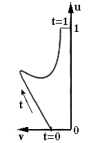Figure 4.6 u,v coordinate system

Example:
The L-System below defines a generalized cylinder of longitudinal length 1.

#define STEPS 0 #define LENGTH 1 Lsystem: 1 derivation length: STEPS Axiom:!(0.4)@Gsf(LENGTH)!(0.2)@Gr(30,4.5,0,3.5)@Ge(20) endlsystem

The longitudinal section is only defined for a segment of unit length. If the segment is not of unit length, the segment can be stretched along the axis.

Example:
The following L-System defines a generalized cylinder of longitudinal length 2.

#define STEPS 0 #define LENGTH 2 Lsystem: 1 derivation length: STEPS Axiom:!(0.4)@Gsf(LENGTH)!(0.2)@Gr(30,4.5,0,3.5)@Ge(20) endlsystem

Notice that the figures can get distorted when the line segment is stretched along the axis. To avoid distortion, the following module can be used:

@Gr(flag)

When the flag=1 in the @Gr module, the tangent vectors keep their angles with the u-axis, thereby avoiding distortion of the image.

Example:
The following L-System defines a generalized cylinder that has it's tangent vectors adjusted.

#define STEPS 0 #define LENGTH 2 Lsystem: 1 derivation length: STEPS Axiom:@Gr(1)!(0.4)@Gsf(LENGTH)!(0.2)@Gr(30,4.5,0,3.5)@Ge(20) endlsystem

If the cylindrical axis is not straight, the longitudinal section is first defined along a straight axis, and then is mapped onto the curved axis.

Example:
The following example illustrates a curved generalized cylinder.
#define STEPS 0 Lsystem: 1 derivation length: STEPS Axiom:!(0.4)@Gs-(45)f-(45)!(0.2)@Gr(30,4.5,0,3.5)@Ge(20) endlsystem

4.3 Modifying the Shape of a Cross Section

4.3.1 Defining a Closed Cross Section

It is possible to override the default disk shape of the cross section of a generalized cylinder by defining a three-dimensional parametric curve consisting of several B-Spline segments. Each control point of a B-Spline segment is represented by three coordinates: an x coordinate, a y coordinate, and a z coordinate. If the cylinder is being produced in a two-dimensional coordinate system, the z coordinate is assigned to be 0.

If n control points are specified, then the contour consists of n B-Spline segments. The parametric B-Spline function Fi(t) is used to compute each segment based on the following four control points: Pi, P(i+1)%n, P (i+2)%n, and P(i+3)%n. The control points of the parametric curve are specified in a text file (see Appendix II).

A certain number of polygons, defined by vertices p, surround the cylindrical mesh strips of generalized cylinders. The required number of vertices on the contour must be found so that the value of p can be set at the beginning of visualization (see Appendix II). The value of p is computed in such a way that the distance between the vertices is approximately constant. Therefore, 10n points on the contour are computed with a constant step of the curve parameter t, where n is the number of control points that specifies the contour. The vertices around the contour are determined by the distances between the points. To connect vertices of different contours, all vertices are rotated around the z-axis in such a way that the first vertex lies on the x-axis[4].

The following module can be used to identify the control points of the different contours:

@#(id)

Example:

The following generalized cylinder has a closed two-dimensional cross section.

#define STEPS 0
#define LEN  2
#define CLEN  0.35
#define BOTTOM 2
#define TOP 2

Lsystem: 1
derivation length: STEPS

Axiom: ,(95)@Tx(1)@#(BOTTOM) #(3)@Gs f(LEN*3)  @#(TOP)@Gc(4) f(CLEN) 

endlsystem

Example:
The following generalized cylinder has a closed two-dimensional cross section that
changes shape as it is swept along the axis.
#define STEPS 1 #define LEN 1 #define CLEN 0.35 Lsystem: 1 derivation length: STEPS Axiom: ,(95)@Tx(1)@#(2) #(3)@Gs f(LEN*3) #(2) @#(0)@Gc(4) f(CLEN) A A --> #(1.0)+(30) f(2*CLEN)@Gc(5) f(LEN) @Ge(4) F(4) endlsystem

Example:
The following generalized cylinder has a closed three-dimensional cross section.
#define STEPS 0 #define LEN 2 #define CLEN 0.35 #define BOTTOM 4 #define TOP 4 Lsystem: 1 derivation length: STEPS Axiom: ,(95)@Tx(1)@#(BOTTOM) #(3)@Gs f(LEN*3) @#(TOP)@Gc(4) f(CLEN) endlsystem

4.3.2 Defining an Open Cross Section

An open contour is defined in the same way as a closed contour is defined. The only difference is in the definition of the control points of a B-Spline segment. For an open contour, n control points specify n-3 B-Spline segments. The B-Spline segments are specified by a B-Spline function Fi(t), t is an element of [0,1], based on the four control points Pi, P(i+1), P(i+2), and P(i+3)[5].

Example:
The following L-System has an open two-dimensional cross section.

#define STEPS 0 Lsystem: 1 derivation length: STEPS Axiom: -(40)@#(2)@Gs-(90)f(10)@Gr(1)@Gr(20,1.5,-20,1.5)@Gt(2,1)-(50)@Ge(20) endlsystem

4.4 Twist of Generalized Cylinders

All vertices of a contour are rotated around the z-axis in the contour coordinate space so that vertices of different contours can be connected. It may happen that in the world coordinate space, between two control points, the turtle's left vector and up vector are rotated around the turtle's heading vector. If the first vertex of the first contour is connected with the first vertex of the second contour, and if the vertices are always aligned with the turtle orientation, then the resulting generalized cylinder will be twisted. By default, the twist in generalized cylinders is minimized, but this minimization can be switched off by a parameter in the view file (see Appendix II).

Example:
The following example shows a twisted generalized cylinder.

#define STEPS 8 Lsystem: 1 derivation length: STEPS Axiom: ,(95)#(2)@Gs A(20) A(n) : n>0 --> f(1)+(4)/(20)@Gc(8) A(n-1) endlsystem

4.5 Branching of Generalized Cylinders

Generalized cylinders produce a branching effect when the following two modules are interpreted:

[

] all turtle parameters are popped off of the stack. This module specifies the end of the stack. The turtle inherits all of the parameters that were popped off of the stack and returns back to the previous state before the branch.

Information about the last control point before the branch is one of the parameters that is saved onto the stack. When a second branch is specified and when the parameters are retrieved, the second branch connects to the last control point that was saved on the stack.

Example:
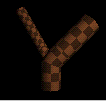
The following example shows a generalized cylinder branching into two or more segments.

#define STEPS 1 #define LEN 1 #define CLEN 0.35 Lsystem: 1 derivation length: STEPS Axiom: ,(95)@Tx(1)#(2)@Gs f(LEN*2) @Gc(4) f(CLEN) A A --> [#(1.0)+(30)f(2*CLEN)@Gc(3)f(LEN)@Gc(4)F(4)]-(45)f(CLEN)@Gc(3)f(LEN)@Ge(4)F(4) endlsystem

					Preface Parameters Appendix I Appendix II References
Index	Circles and Spheres	Generalized Cylinders	Surfaces	Textures